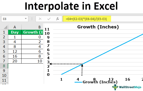
How to Interpolate in Excel

Interpolation is a mathematical tool used to estimate values that are not directly available in a dataset. Excel provides an easy way to perform interpolation through its powerful formula ecosphere. After analyzing a large set of data, users are likely to encounter missing values that would have otherwise provided critical information for their analysis. In such a scenario, the best option is to perform interpolation and estimate the missing values.
Interpolation can be done through various methods, including linear interpolation, polynomial interpolation, and spline interpolation. In Excel, simple linear interpolation is the most commonly used method. It can be done in four simple steps, as follows:
1. Identify the target cell where the interpolated value should be placed.
2. Identify the cells that contain the data that needs to be interpolated. The data must be arranged in two columns, with the first column containing the independent variable and the second column containing the dependent variable.
3. Use the LINEST function to calculate the slope and the intercept of the line that connects the two points that lie closest to the target cell. The syntax for the LINEST function is as follows:
=LINEST(known_y’s, known_x’s)
Where known_y’s specifies the dependent variable column, and known_x’s specifies the independent variable column.
4. Use the slope and the intercept values obtained in step 3 to calculate the interpolated value of the target cell. The formula is as follows:
=intercept + (target cell’s independent value – closest point’s independent value) * slope
Where intercept is the value obtained from the LINEST function in step 3, and the closest point is the point that lies immediately above or below the target cell.
Example:
Suppose a dataset contains the following values:
Independent variable | Dependent variable
—————————-
10 | 4
20 | 8
30 | 12
40 | ?
The value in the fourth row needs to be interpolated.
Step 1: Identify the target cell where the interpolated value should be placed. In this case, it is the cell containing the missing value.
Step 2: Identify the cells that contain the data that needs to be interpolated. In this case, it is the first and second column.
Step 3: Use the LINEST function to calculate the slope and the intercept of the line that connects the two points that lie closest to the target cell. The syntax for the LINEST function is:
=LINEST(B2:B4, A2:A4)
Where B2:B4 specifies the dependent variable column, and A2:A4 specifies the independent variable column.
The output is:
Slope | Intercept |
————
4 | 0
Step 4: Use the slope and the intercept values obtained in step 3 to calculate the interpolated value of the target cell. The formula is:
=intercept + (target cell’s independent value – closest point’s independent value) * slope
=0 + (40-30) * 4
= 16
Therefore, the interpolated value of the missing cell is 16.


